Huygens’ Surfaces
Yankun (Alex) Meng
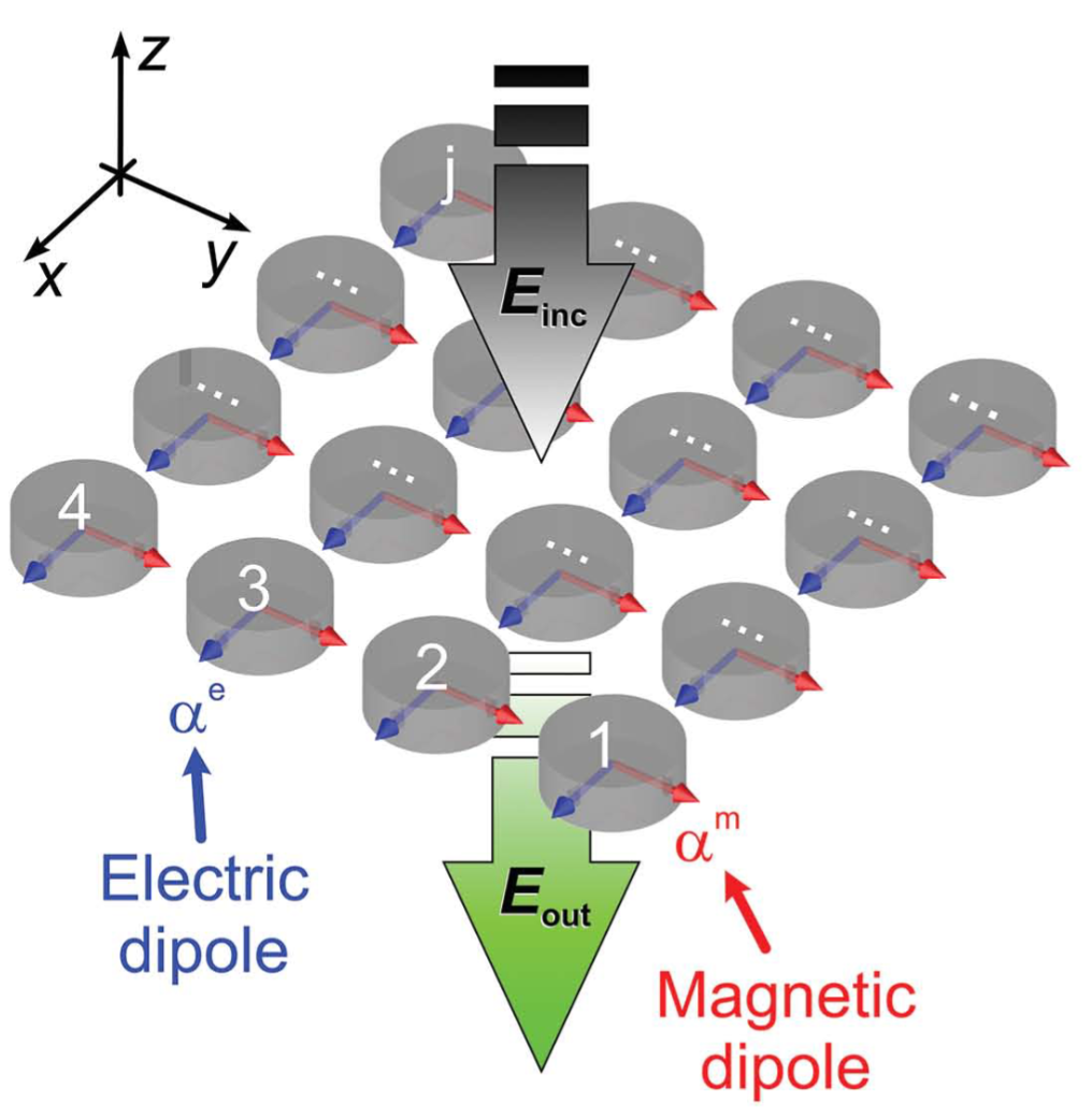
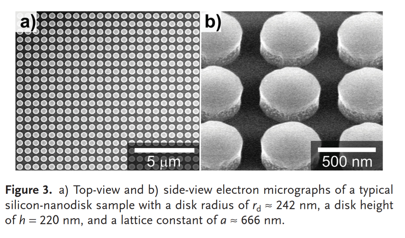
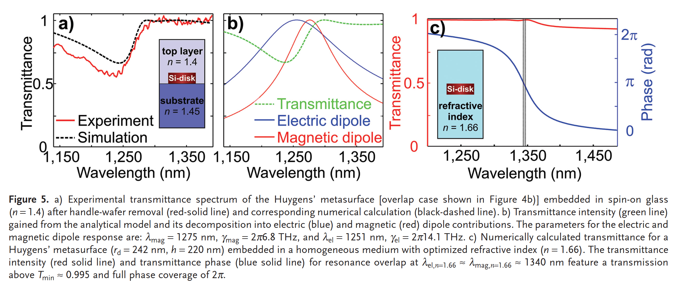
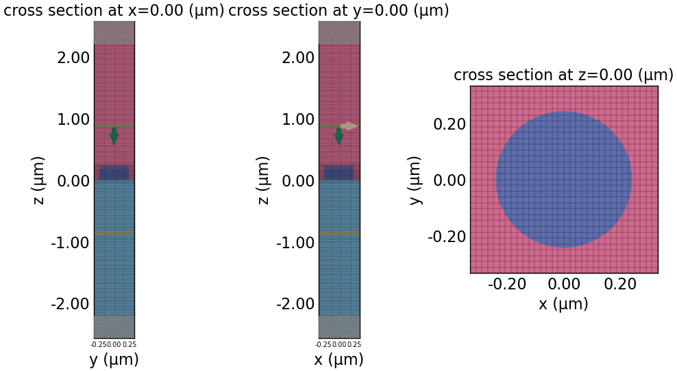
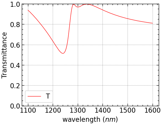
In this notebook, the Huygens’ Metasurface figure 5(a) and 5(c) are reproduced, and mesh study is done for the transmittance. Link to Paper
Simulation 1
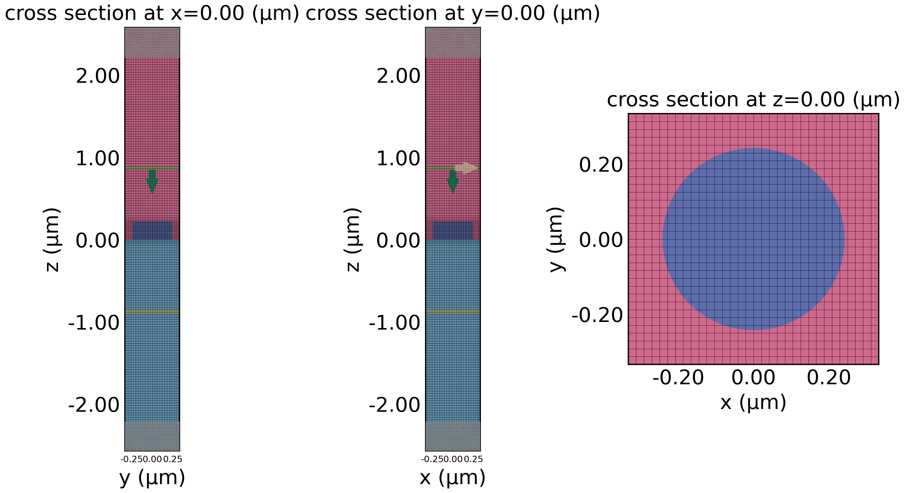
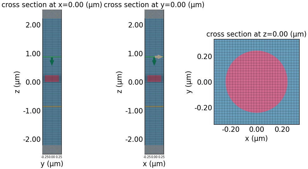
Top Layer n=1.4, Bottom Layer n=1.45
Simulation 2

Background medium n=1.66
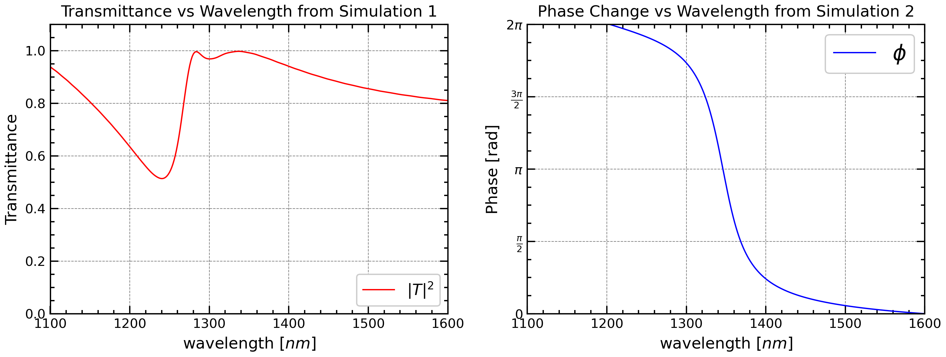
Simulation Results
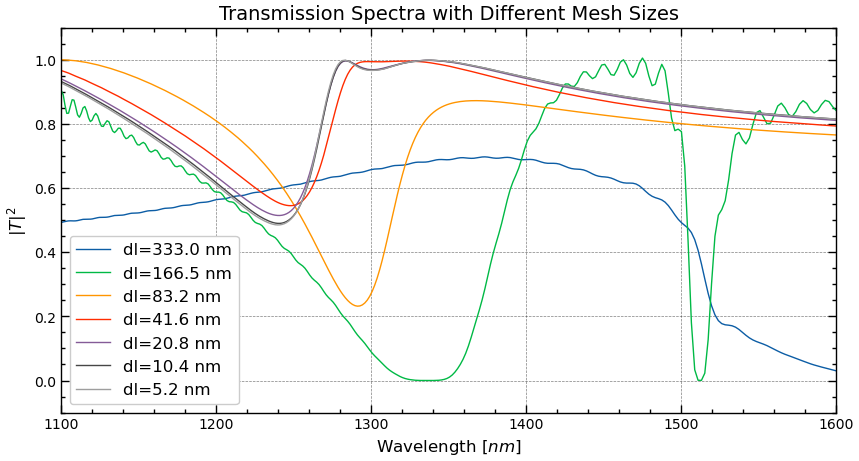
Mesh Study Results
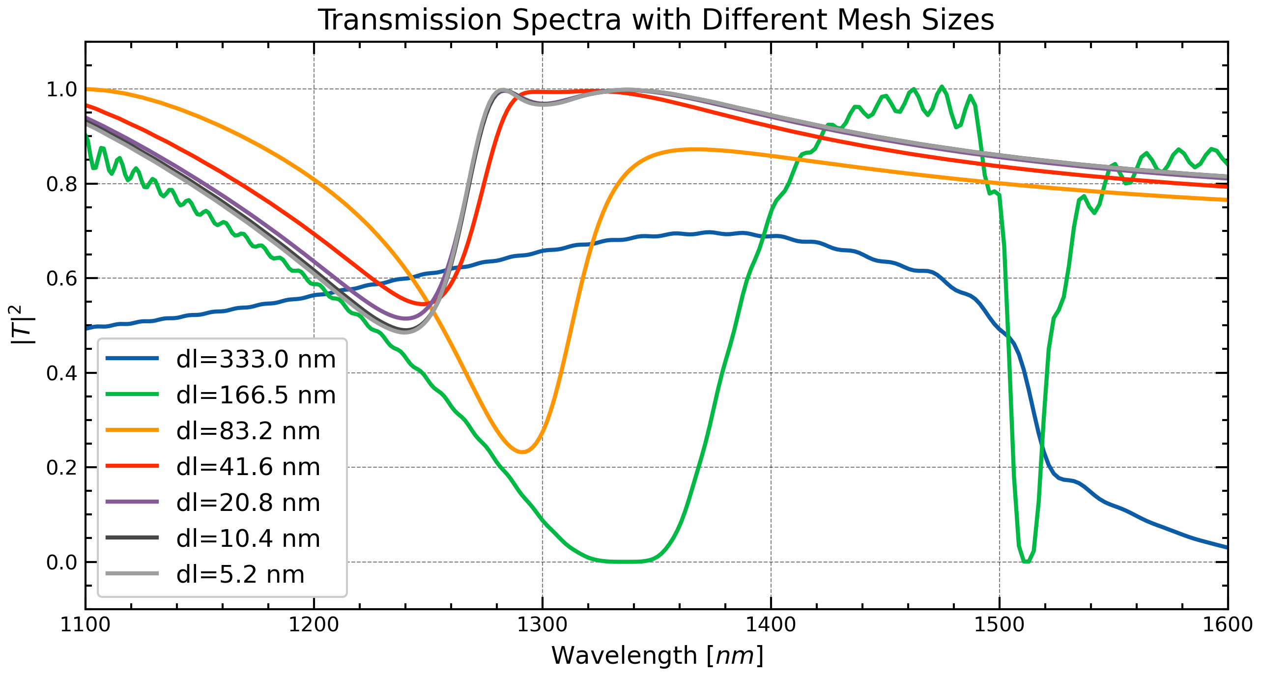
Convergence of Transmittance
Transmittance Simulation
02:20:56 EDT Started working on Batch containing 2 tasks.
02:20:57 EDT Maximum FlexCredit cost: 0.050 for the whole batch.
             Use 'Batch.real_cost()' to get the billed FlexCredit cost after the
             Batch has completed.
02:20:58 EDT Batch complete.
Transmittance Results
Phase Simulation
02:21:11 EDT Started working on Batch containing 2 tasks.
02:21:13 EDT Maximum FlexCredit cost: 0.050 for the whole batch.
             Use 'Batch.real_cost()' to get the billed FlexCredit cost after the
             Batch has completed.
02:21:14 EDT Batch complete.
Phase Results
# 1. Compute average over the xy-plane
Ex_avg = np.mean(Ex[:, :, 0, :], axis=(0,1))

# 2. Compute phase
phase_avg = np.angle(Ex_avg)

# 3. Unwrap phase to remove ±pi jumps
phase_avg_unwrapped = np.unwrap(phase_avg)

# 4. Make relative to first point (optional)
phase_rel = phase_avg_unwrapped - phase_avg_unwrapped[0]

phase_actual = np.unwrap(np.angle(np.mean(Ex_actual[:, :, 0, :], axis=(0,1))))
phase_norm = np.unwrap(np.angle(np.mean(Ex_norm[:, :, 0, :], axis=(0,1))))
fig, ax = plt.subplots(1, 1, figsize=(6, 4.5))
plt.plot(td.C_0 / fr.freqs(N) * 1000, phase_rel, "r", lw=1, label="$\phi$")
plt.plot(td.C_0 / fr.freqs(N) * 1000, phase_actual, "b", lw=1, label="Actual $\phi$")
plt.plot(td.C_0 / fr.freqs(N) * 1000, phase_norm, "g", lw=1, label="Norm $\phi$")
plt.xlabel(r"wavelength ($nm$)")
plt.ylabel("Phase")
plt.legend()
plt.show()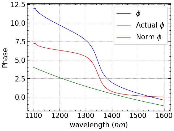
Final Plotting
fig, axes = plt.subplots(1, 2, figsize=(12, 4))

# work on the first figure
ax = axes[0]
ax.tick_params(axis="both", labelsize=10)
ax.plot(td.C_0 / fr.freqs(N) * 1000, np.abs(T)**2, "r", lw=1, label="$|T|^2$")
ax.set_xlabel(r"wavelength [$nm$]", fontsize=12)
ax.set_ylabel("Transmittance", fontsize=12)
ax.set_title("Transmittance vs Wavelength from Simulation 1", fontsize=12)
ax.set_xlim(1100, 1600)
ax.set_ylim(0, 1.1)
ax.legend(loc="lower right", fontsize=12)

# work on the second figure
ax = axes[1]
ax.tick_params(axis="both", labelsize=10)
ax.plot(td.C_0 / fr.freqs(N) * 1000, phase_rel, "b", lw=1, label="$\phi$")
ax.set_xlabel(r"wavelength [$nm$]", fontsize=12)
ax.set_ylabel("Phase [rad]", fontsize=12)
ax.set_title("Phase Change vs Wavelength from Simulation 2", fontsize=12)
ax.set_xlim(1100, 1600)
ax.set_ylim(0, np.pi*2)
yticks = [0, np.pi/2, np.pi, 3*np.pi/2, 2*np.pi]
ytick_labels = [r"$0$", r"$\frac{\pi}{2}$", r"$\pi$",
                r"$\frac{3\pi}{2}$", r"$2\pi$"]
ax.set_yticks(yticks)
ax.set_yticklabels(ytick_labels)
ax.legend()

plt.savefig("huygens.png", dpi=300)
Mesh Study Results
# Plot results
plt.figure(figsize=(10, 5))
for i, T in enumerate(Ts):
    plt.plot(x, np.abs(T)**2, "-",lw=1, label=f"dl={dls[i] * 1000:.1f} nm")
plt.xlabel(r"Wavelength [$nm$]", fontsize=12)
plt.ylabel(r"$|T|^2$", fontsize=12)
plt.xlim(1100, 1600)
plt.ylim(-0.1, 1.1)
plt.legend(fontsize=12)
plt.tick_params(axis='both', labelsize=10) # change tick label size to 10
plt.title("Transmission Spectra with Different Mesh Sizes", fontsize=14)
plt.savefig("mesh_convergence.png", dpi=300)
plt.show()